Getting started
This section provides a quick start guide to the AIXD toolkit. Here, we illustrate the fundamental capabilities of the AIXD toolkit using a straightforward analytical example. The example serves as a domain-independent introduction, chosen for its simplicity and the clear visualization of the toolkit’s functionalities.
The notebook for this example can be found in the example section.
In this introductory example, we demonstrate how to use the toolkit to formulate the design problem, create a dataset and train and deploy a model.
1. Definition of parametric problem
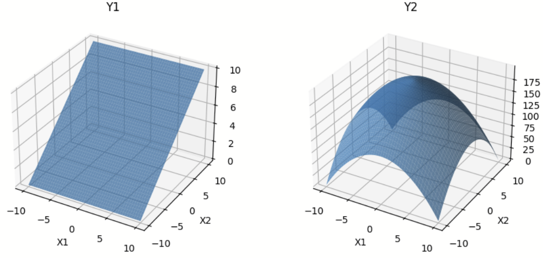
As a simple example, we will train neural network models to learn two analytical functions \(Y_{1}\) and \(Y_{2}\) dependent on two real-valued variables \(X_{1}\) and \(X_{2}\). These functions are defined as follows:
def analytical_function(X1,X2):
    Y1 = 0.5*X2 + 5
    Y2 = -(X1**2 + X2**2) + 200
    Y = np.array([Y1,Y2])
    return Y
2. Dataset creation
Define your design parameter and performance attributes
Our DesignParameters are therefore \(X_{1}\) and \(X_{2}\), and our PerformanceAttributes \(Y_{1}\) and \(Y_{2}\). First we need to define the corresponding Data Objects. All of them are real-valued, hence we define them as DataReal objects, and an Interval as their domain.
from aixd.data.data_blocks import DesignParameters
from aixd.data.data_objects import DataReal
from aixd.data.domain import Interval


# Define design parameters
obj_list = [DataReal(name='x1', dim=1, domain=Interval(-10, 10)),
            DataReal(name='x2', dim=1, domain=Interval(-10, 10))]

design_parameters = DesignParameters(name='design_par', dobj_list=obj_list)
And similar we define the performanceAttributes:
from aixd.data.data_blocks import PerformanceAttributes

obj_list=[
    DataReal(name="y1", dim=1) ,
    DataReal(name="y2", dim=1),
    ]
performance_attributes = PerformanceAttributes(name='perf_att', dobj_list=obj_list)
Create your Dataset object
Using the defined DesignParameters and performanceAttributes, we initialize the Dataset object. Here we just define the structure of the Dataset - it does not contain any data yet.
from aixd.data.dataset import Dataset

dataset = Dataset(root_path = None,
                    name="analytical_example",
                        design_par=design_parameters,
                        perf_attributes=performance_attributes)
The data will be stored in prescribed subfolders under the root_path - if None is specified, the current working directory will be used by default.
Import data to your Dataset object
If we have data available we can simply import our data into the Dataset. Here we import the data from a pandas DataFrame into our Dataset object that we have created before.
dataset.import_data_from_df(df)
Sample the design space, analyze and save to data set
Skip this section if you already have data you want to train your model on, and you managed to import the data to the Dataset using the above import function.
However, if you don’t have your data yet and want to use the built-in methods to sample your data this section is helpful.
We have already defined our design parameter space for this example. We can now sample this design space to get our design parameter vectors:
n = 10000
batchsize = 1000
dataset.sampling(n_samples=n, samples_perfile=batchsize, strategy="uniform", engine="random")
To evaluate our samples we have to define our custom analysis pipeline. In this example this is simply evaluating the analytical function for all the sampled design parameter vectors:
def analysis_pipeline(input=None):

"""
Project-specific & user-defined analysis function.
Here we evaluate a pandas DataFrame with the defined analytical functions.

Parameters
----------
data: pd.DataFrame
    A DataFrame with design parameters. Each row represents one design sample.

Returns
-------
np.array[float,int]
"""


result = input.apply(lambda row: analytical_function(row[['x1', 'x2']].to_numpy()),axis=1)
Y = np.array(result.tolist())


return Y
Once this analysis_pipeline() function is defined for the specific problem, we can evaluate all samples. Here we first create our analysis class and then analyze our samples.
from aixd.data.custom_callbacks import AnalysisCallback

analyzer_class = AnalysisCallback('Analysis', func_callback = [analysis_pipeline], dataset = dataset)
dataset.analysis(analyzer = analyzer_class)
By default this function saves the samples and their analysis results. We can check the saved data for example by looking at the DesignParameters and performanceAttributes in the Dataset:
dataset.data['design_parameters'].head()
dataset.data['performance_attributes'].head()
For further exploration of the generated or imported data we can plot the data or use further built in data exploration functions of the AIXD toolkit (see next section).
3. Data exploration
Next we can use the data visualization functionalities of the Plotter to understand our data. For that we need to set up our Plotter object.
from aixd.visualisation.plotter import Plotter

plotter = Plotter(dataset, output='plot')
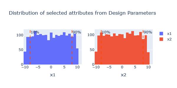
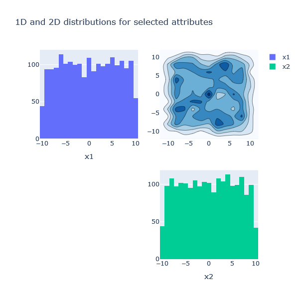
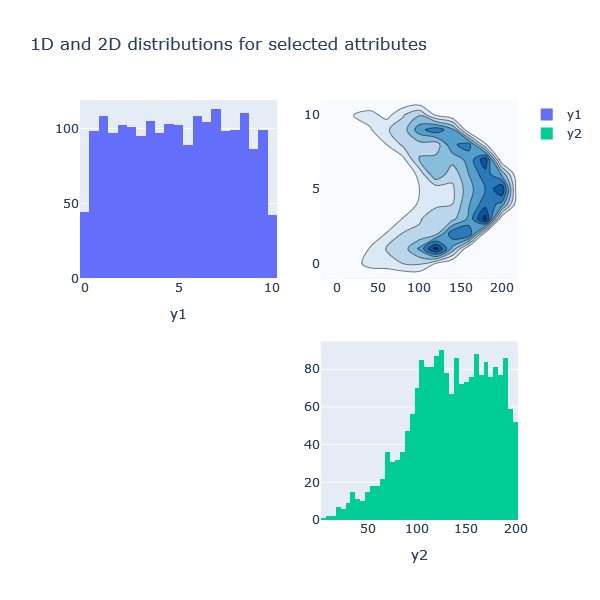
Helpful is for example to visualize the variable distributions.
plotter.distrib_attributes(block='design_par', per_column=True, sub_figs=True)

plotter.distrib_attributes(blocks=['performance_attributes'], per_column=True, sub_figs=True)
plotter.contours2d(block='design_par')
plotter.contours2d(block='perf_att')
3. Model set-up, training and evaluation
Set-up
The next step is to set-up the Machine Learning Model. In this example we train a conditional autoencoder to be able to function both as a surrogate model (for an input \(X\) predicting \(Y\)) as well as an performance-oriented generative model (for defined constraints for \(Y\) generate valid \(X\)).
First we define the input and output of our model. In this case the inputs are our DesignParameters (\(X\)) and our outputs the performanceAttributes (\(Y\)).
inputML = dataset.design_par.names_list
outputML = dataset.perf_attributes.names_list
Next, we need to create a DataModule from our Dataset.
from aixd.mlmodel.data.data_loader import DataModule

datamodule = DataModule.from_dataset(dataset, input_ml_names=inputML, output_ml_names=outputML, batch_size=1000)
Now, we can define the structure of our Model. We first import the model we want to train and then initialize this model from our DataModule. We here define the number of layers (here: 3) and the individual widths of each layer (here: 16,8,4). Furthermore the number of latent dimensions has to be chosen (here:1).
from aixd.mlmodel.architecture.cond_ae_model import CondAEModel

cae = CondAEModel.from_datamodule(datamodule, layer_widths= [16, 8, 4], latent_dim=1)
The Model we have defined above is a conditional autoencoder and has the following visualised structure:
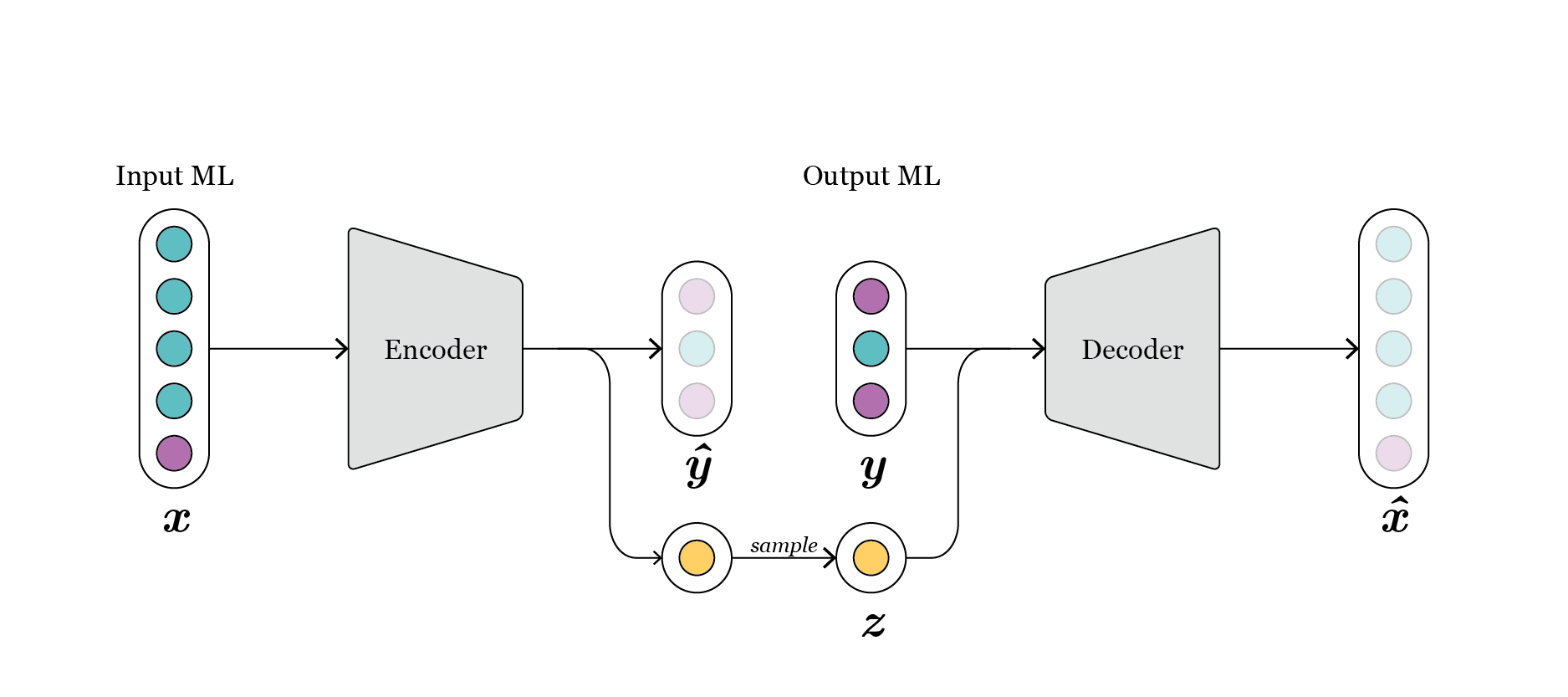
Fig. 1: schematic representation of vanilla conditional-autoencoder.
Training
Now that the Model structure is set-up we train the model. Meaning we fit the Model to our training data. Here we select to train maximum for 100 epochs and turn on early stopping.
import warnings

with warnings.catch_warnings():
    warnings.simplefilter('ignore', category=UserWarning)
    cae.fit(datamodule, name_run='Run1', max_epochs=100, flag_early_stop=True)
For more guidance and explanations on how to setup and training different neural network models, please refer to the setup and training section of this documentation.
Evaluation
The third step of this chapter is the evaluation of the trained Model. We first import the Model and then visually evaluate it. The Model evaluation is important, in order to discern how successful the training has been, and if the architecture may benefit from changes.
To load the trained Model we just need to provide the path to the checkpoint.
path = f'{dataset.datapath}/{CondAEModel.CHECKPOINT_DIR}/last.ckpt'
cae = CondAEModel.load_model_from_checkpoint(path)
To visually evaluate the trained Model we have multiple helpful functionalities in the Plotter. First we need to initialize the Plotter again. This time additional to the Dataset we also need to provide the Model that we want to evaluate to the Plotter object.
from aixd.visualisation.plotter import Plotter

plotter = Plotter(dataset=dataset, model=cae)
The below figure shows the predicted values Plotter against the true values from the validation Dataset. A perfect fit would mean that all scatter points lie on the 45° line. By normalizing the data we archive the error in the original units.
plotter.attributes_obs_vs_pred(block="outputML", datamodule=datamodule,transformed=False, n_cols=2)

Another helpful visualisation is gained by the evaluate_training() function:
plotter.evaluate_training(datamodule=datamodule, attributes=['y1'],transformed=False, bottom_top=(0.1, 0.9))
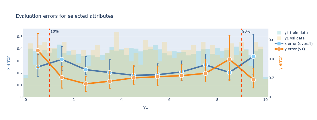
plotter.evaluate_training(datamodule=datamodule, attributes=['y2'],transformed=False, bottom_top=(0.1, 0.9))
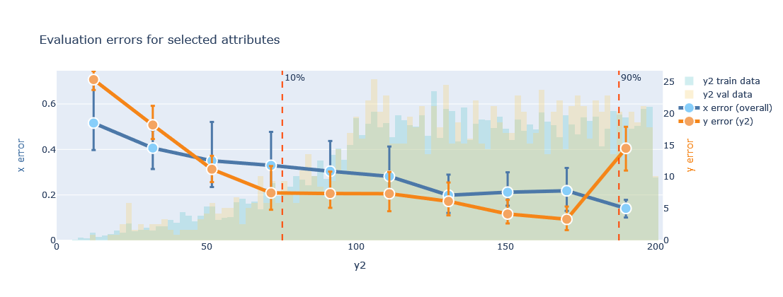
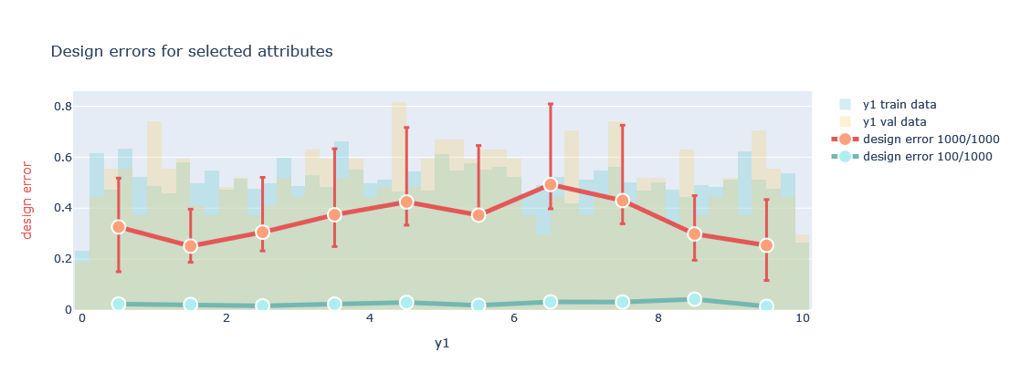
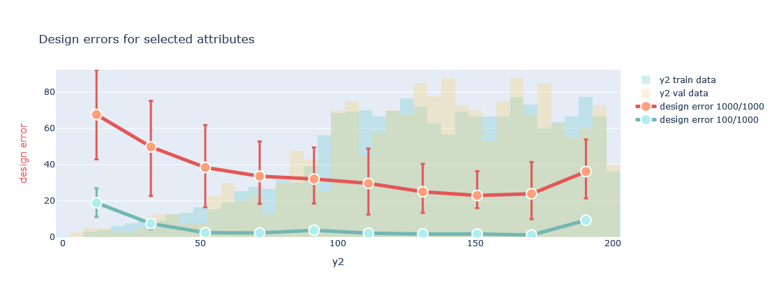
Additionally we can also look at the generative design error the trained Model makes.
plotter.evaluate_generation(datamodule=datamodule, attributes=['y1'],transformed=False)
plotter.evaluate_generation(datamodule=datamodule, attributes=['y2'],transformed=False)
For detailed guidance on using these plots and interpreting their results, please refer to the model evaluation section of this documentation.
5. Model deployment
Once the Model is trained and evaluated, it can be deployed to the respective design problem. Below we show how the trained Model can be used to (i) inversely generate new samples based on defined constraints and (ii) evaluate a large amount of samples in quasi-real time.
Inverse Design: Constrained Generation
Our goal here is to use the trained Model to generate new samples, while considering defined performance constraints. We refer to this operation as the Inverse Design.
We first need to initialize our Generator. You need to provide the trained Model and the DataModule.
from aixd.mlmodel.generation.generator import Generator

gen = Generator(model = cae, datamodule = datamodule)
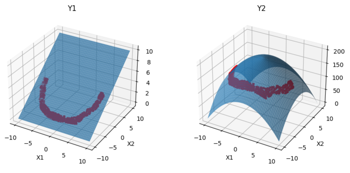
To make an example we want to generate samples which have a \(Y_{2}\)-value between 135 and145. To execute this generation we first need to formulate this request in a dictionary, and then provide it to the generator. Here we chose to generate 1000 samples, and the output type DataFrame.
request={'y2': [135,145]}
df_gen, _ = gen.generation(request, n_samples = 1000, format_out='df')
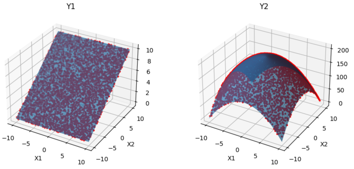
When we visualize the generated data we can see a clear line at the selected performance range.
But we can not only condition on a single attribute, but on multiple attributes at the same time.
request={'y1':[0,5], 'y2': [135,145]}
df_gen, _ = gen.generation(request, n_samples = 1000, format_out='df')
Forward Design: Prediction
We can also use the encoder Model to evaluate a large amount of samples in quasi-real time. This can be beneficial for example for the optimisation of the design.
To show this functionality we here import a large amount of design parameter vectors from a csv-file to be evaluated by the trained encoder.
df = pd.read_csv('analytical_function_samples.csv')

df_pred=cae.forward_evaluation(df[['x1','x2']], format_out="df")
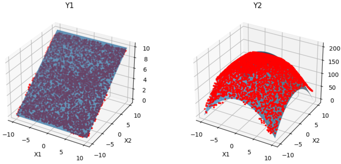
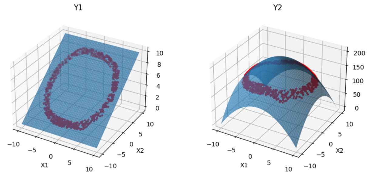
If we plot the predictions made by the encoder against the actual surfaces of the analytical function we can see that the Model learned the surfaces accurately.
