ML-Model

The machine learning model, based on neural networks, is the backbone of the current toolbox, as it allows carrying out forward evaluation and inverse design. It can be easily defined, provided the Dataset object, and then trained using the contained data. Once trained, it is leveraged to perform generative design, as well as a surrogate model of the CAD or finite element model. In the following sections, we provide more details about the models used, as well as its usage

Autoencoder architecture

We rely on an autoencoder (AE) architecture, composed of an encoder and a decoder stage. This architecture fits ideally the problem at hand because, once the model is trained, the encoder is a surrogate model of the design and analysis pipeline, and the decoder can be leveraged to perform inverse design. In Fig. 1 we depict the different elements that form the model. With \(x\) we refer to the design features that uniquely define a geometry, and with \(y\) to the associated performance attributes, computed using CAD or FEM methods. Besides, to capture the fact that different sets of design features can lead to similar values of performance attributes, the latent feature \(z\) captures the degrees of freedom. In generative design application, the user only needs to specify the values of \(y\) they want their design to fulfill. Then, the model samples \(z\), and concatenates vectors \([y,z]\) passed to the generator to obtain sets of design features that approximate the provided request \(y\).

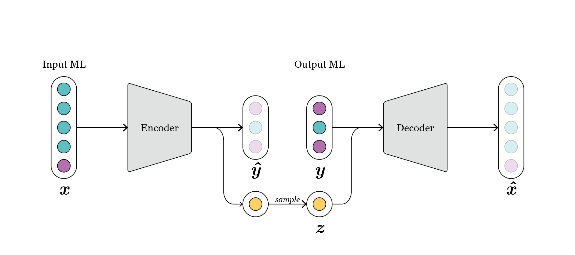
Fig. 1: schematic representation of vanilla conditional-autoencoder.

In the toolbox we have implemented two well-known neural network architectures to carry out the learning: a conditional autoencoder (CAE) and a conditional variational autoencoder (CVAE).

In the basic architecture, a “vanilla” conditional-autoencoder (CAE) (Fig. 1), each \(x\) is mapped to an estimation of its respective associated performances, \(\hat{y}\), and some specific values in the latent dimension \(z\). The latent feature is regularized to have zero mean and unit variance, such that the distribution of \(z\) approximates Gaussian distribution. This enables easily sampling the space of \(z\) during the generation phase.

Besides, we implement a conditional variational autoencoder (CVAE) [Kingma2013] [Sohn2015] (Fig. 2). In this case, the distribution of \(z\) in the latent space is also enforced to approximate a multivariate Gaussian distribution. However, in this case a reparametrization trick is used, and instead of mapping \(x\) directly to samples in the space \(z\), the distribution \(z\) is represented through its sufficient statistics, mean and variance, and \(x\) is mapped to them. During training, the loss term enforces these sufficient statistics to approximate a zero mean and unit variance Gaussian. During generation, we just need to sample this Gaussian distribution, concatenate with \(y\), and propagate it through the decoder to get new designs.

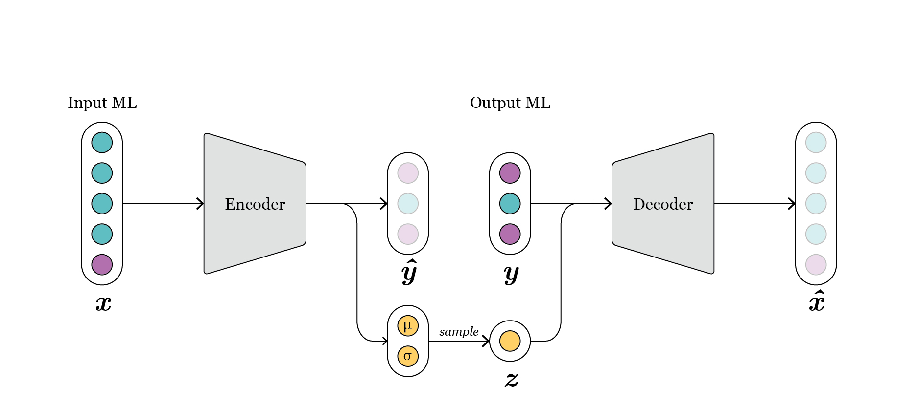
Fig. 2: schematic representation of conditional variational-autoencoder.

Besides, all models are characterized by some features that define the architecture. First, the number of layers specify the number of linear transformations applied during encoding and decoding. Each of these linear transformations is followed by a non-linear activation function, such as Relu or Leaky-Relu, being the latter the default one. Additionally, each of this layers is characterized by the number of neurons, i.e. its dimensionality. Hence, the final number of parameters is a function of the number of layers and their dimensionalities, and therefore are the main hyperparameter to be tuned.

Setup and training

To carry out the definition and usage of the machine learning (ML) model, we need first a Dataset instance, as this includes all the information about DesignParameters and PerformanceAttributes, and DataObjects contained within. Now, the process of defining, training and evaluating the learning model can be superficially described as follows: 1. Define inputs and outputs for the ML model, as well as normalizations (optional). 2. Create the DataModule 3. Set up the model by choosing the type, number of layers, etc. 4. Run the training.

In the following sections, we will dig deeper into each of these steps, providing also snippets that can be directly utilized in other use cases.

Definition of InputML and OutputML

In a nutshell, the ML model learns a mapping between some certain input \(x\) (we denote it here as InputML) and its associated \(y\) (OutputML). Besides, \(x\) is mapped to a latent space \(z\). The simplest scenario is when \(x\) and \(y\) correspond one to one with the DesignParameters and PerformanceAttributes. This is just specified by providing the list of names (strings) of all DataObjects as follows:

# Input and output ML match one to one the design parameters and performance attributes
inputML_names = dataset.design_par.names_list
outputML_names = dataset.perf_attributes.names_list

Where the internal variables names_list is used to retrieve the list of strings.

Furthermore, the toolbox allows to specify any possible mapping for the ML model. In order to define it, we just have to provide a different list of DataObject names, for example:

# Input and output ML match one to one the design parameters and performance attributes
dp_objects = dataset.design_par.names_list
pa_objects = dataset.perf_attributes.names_list
inputML_names = dp_objects[:5] + [pa_objects[0], pa_objects[3]]
outputML_names = dp_objects[5] + pa_objects[1:3]

This possibility can be of interest in use cases where, even though some parameters are part of the definition of the geometry, e.g. the height, still we would like to utilize them for the generation of new geometries.

In Fig. 3 we observe the configuration of design parameters and performance attributes, as indicated by the colors, in the original parametric model. At the time of defining the ML model, we can consider a diferent mapping, as illustrated in Fig. 4.

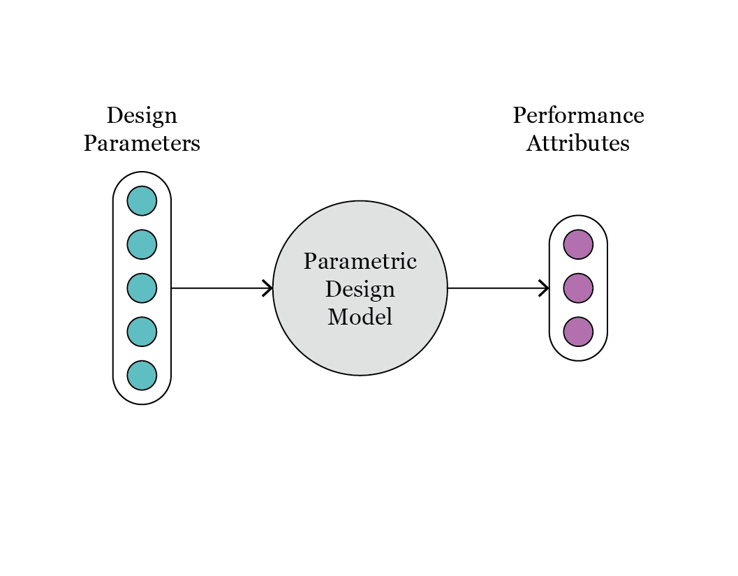
Fig. 3: schematic representation of the original parametric model, with design parameters and performance attributes.

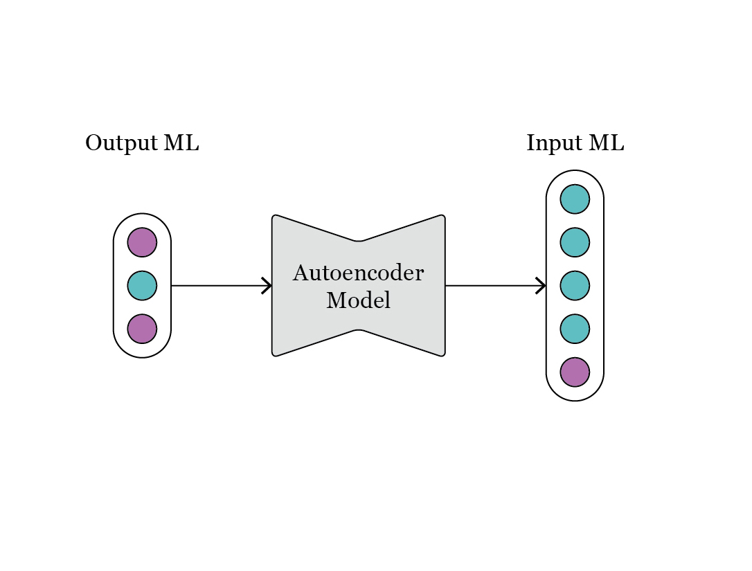
Fig. 4: representation of the mapping between OutputML and InputML, as requested during the step of generative design.

Additionally, different normalization and transformation functions can be defined for each data object. In order to do it, we have to assign the normalization/transformation of interest to each respective DataObject as follows:

# Definition of standard, i.e. zero mean and unit variance, normalization of some data objects in the design parameters block
dataset.design_par.dobj_list[0].transformations = ["standard_scaler"]

You can define normalizations for a subset, or all, DataObjects:

# Definition of standard, i.e. zero mean and unit variance, normalization of some data objects in the design parameters block
dataset.design_par.dobj_list[:5].transformations = ["norm_0to1"]
dataset.perf_attributes.dobj_list[:].transformations = ["standard_scaler"]

Transformation (more details in API) functions are applied to the data before being fed to the ML model, in order to provide a more amenable representation. By default, DataReal and DataInt objects are normalized to a range 0 to 1 (norm_0to1), while for categorical and ordinal data objects a label encoder is applied to transform strings to integer labels. A list of all possible transformations can be printed with print(aixd.data.transform.list_transformations()).

Creation of datamodule object

The DataModule class is a subclass of the corresponding PyTorch Lightning datamodule class (i.e., LightningDataModule). It can be created seamless by the classmethod DataModule.from_dataset(...) by just providing the Dataset instance with additional optional arguments. The following snippet illustrates the creation of the DataModule object:

from aixd.mlmodel.data.data_loader import DataModule
# Creating the DataModule required by PyTorch
datamodule = DataModule.from_dataset(dataset, input_ml_names=inputML_names, output_ml_names=outputML_names, batch_size=256)

While the batch_size in principle should be as large as the GPU/CPU memory allows, some additional hints to select it can be found in [Keskar2016].

Internally, the DataModule object creates two new data blocks: input_ml_dblock and output_ml_dblock. These inherit the data objects from the Dataset as indicated by the parameters input_ml_names and output_ml_names. The DataModule contains several methods to call the dataloaders required by the neural network, and to obtain the different data splits, i.e. train, validation and test.

In principle, all users will only be required to call this method once to generate a Datamodule instance, as presented above.

Definition of ML model

The model class for both architectures defined above, i.e. a conditional AE and a conditional variational AE, are built on top of the LightningModule model class from PyTorch Lightning. The subclasses CondAEModel and CondVAEModel receive all the information required to define the losses, layers, etc., from the DataModule instance created before. Nevertheless, the user still needs to provide some additional information for the creation of the neural network: the number of layers with their dimensionality, and the dimension of the latent space. One example of the creation of the model is presented in the following:

from aixd.mlmodel.architecture.cond_ae_model import CondAEModel
# Create the model based on the data module
cae = CondAEModel.from_datamodule(datamodule, layer_widths=[512, 256, 128, 64], latent_dim=30, save_dir=<my_datapath_for_checkpoints>)

Where <my_datapath_for_checkpoints> is the folder where the checkpoints folder will be created. For convenience, you can just refer to the datapath of the dataset as follows dataset.datapath.

It is not trivial to define the layer_widths parameter, as it depends on different factors such as the dimensionality of the input, the number of samples in the dataset, etc. Typically, the latent dimension is considerably smaller than the input dimensionality in order to create a bottleneck between the encoder and the decoder. For example, the definition above corresponds to a scenario where we start with an input dimensionality, i.e. that of InputML, of 630. Hence, we choose the first layer to have dimensionality 512. We decide to reduce the dimensionality to 30 in the latent space \(z\). This is added up to the dimensionality of OutputML, in this case 8, leading to a total of 38. For this reason, the last layer is assigned a size of 64. Besides, in addition to the two layers of dimensionality 512 and 64, we define 2 additional layers with dimensionality 256 and 128. We believe this leads to an adequate size for the neural network given the large size of the dataset (around 100 thousands samples). From the previous example, we can conclude that, as a rule of thumb, the first layer may have a dimensionality around the input dimensionality, and then create a progressive bottleneck towards the latent space. The latent space requires a much lower dimensionality than the input dimensionality, but should still be able to encode the degrees of freedom.

The previous selection of parameters for the network is still an educated guess. In principle, the users should perform a more thorough process of model selection to determine the best architecture of the model (e.g. number of hidden layers, hyperparameters). Currently, for model selection, the user needs to manually run different training experiments, with different definitions of the model architecture, and evaluate which is the best performing one. However, in future releases, we will implement automatic procedures to automatically tune these parameters.

Training the ML model

Now we can easily start different training campaigns, just calling the fit method of the model.

# If the training is run in a notebook, different warning might be generated, leading to a quite verbose output
import warnings
with warnings.catch_warnings():
    warnings.simplefilter('ignore', category=UserWarning)
    cae.fit(datamodule, name_run='Experiment 1', max_epochs=50, accelerator='gpu', flag_wandb=False)

We can provide callbacks as those used in the trainer method of PyTorch Lightning, and set a criteria for early stopping through the parameters flag_early_stop and criteria. Besides, if flag_wandb=True, a default Weight and Biases logger is invoked . The results of an experiment are saved in a checkpoint file, stored by default in folder <save_dir>/checkpoints/.

Evaluating the performance of each training experiment

There are different ways to assess the performance of the trained model and compare against other trained models. Many of these are complementary, and can help understanding the results. In a nutshell, we can analyze the results from three points of view:

1. Compare different trained models by analyzing their losses. This we can just do by using the results prompted when running the fit method of the model class. However, it is more efficient to use Weight and Biases as the logger for the results by activating the flag flag_wandb=True. The intuitive dashboard of WandB enables us to easily compare the performance of different experiments, in order to select the best for the subsequent steps. All losses are logged, and can be intuitively plotted, smoothed, etc. However, as we will see with next comparison methods, a better evaluation loss, specially if it is just a tiny improvement, does not mean a better model for both tasks of forward prediction and inverse design.

2. Assess the quality of the training using some methods integrated in the plotter. With the method evaluate_training, we can visualize the performance of reconstruction loss for \(x\), and the quality of the forward model as induced by individual attribute(s) in OutputML \(y\):

plotter.evaluate_training(datamodule=datamodule, attributes=['y2'], transformed=True, bottom_top=(0.1, 0.9))

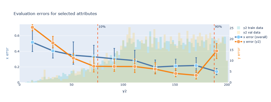
The results can be plotted using transformed values (normalize=transformed) or in their original domain (transformed=False). Besides, the distribution of the attribute is plotted in the background of the line plot, to examine if the training is indeed better in areas with more data points. The \(x\) error may be difficult to interpret, as it can combine losses for real and categorical variables. However, the \(y\) error for the indicated attribute provides an intuitive view of the quality of the forward model. In the exemplary plot shown above, the \(y2\) attribute has values in the range 0 to 200, with a larger concentration of samples above 100. For almost all this range, the error of \(y2\) is below 5, so less than 5% for all cases.

We can also evaluate the performance of the trained model using the scatter plot implemented in the plotter. This allows comparing the ground truth values of \(x\) and \(y\) versus the predicted. The call of the methods and the results look as follow:

plotter.attributes_obs_vs_pred(block="outputML", datamodule=datamodule, transformed=False, n_cols=2)

3. Probe the model to understand its generation capabilities by looking at the design error defined as:

\[error\_design = |y^* - \hat{y}|\]

The variable \(y^*\) refers to the specific value requested by the user for a certain attribute. If the request is a range, the error will be 0 for all \(y\) falling inside the range. Otherwise, the error is computed from the mean value of the specified range. Then, \(\hat{y}\) refers to the prediction of the encoder for all designs provided by the decoder. However, given that the encoder is just a surrogate model of the ground truth analysis pipeline, \(\hat{y}\) is just an estimate, and can deviate from the true \(y\) value for a certain design \(x\). Therefore, when interpreting the following results, the user also needs to take into account the results of those methods explained in 2, as these are an indicator of the performance of the encoder as a surrogate model.

plotter.evaluate_generation(datamodule=datamodule, attributes=['y2'], transformed=False)

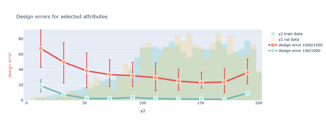
In this plot, for the selected attribute from OutputML, and for different bins of its distribution, the method generates a number of designs for values within each bin and calculates the design error. The line plot shows the mean and variance of this error for all the designs generated (red), and the best 10% of designs, selected using predictions of the encoder (green). These plots help to elucidate in which areas of the attributes the generated designs better approximate the requested values. Therefore, it helps understanding the quality of the designs we can expect, and if we can leverage already the trained model to start exploring the space of solutions.

Model application

By following the steps described above, the user can easily create a model and train it. Even though it is desirable to carry out a thorough campaign of hyperparameter tuning, i.e. adjustment of the model parameters, most models will allow carrying out an exploration of the solution space, the discovery of novel solutions, and its usage as a surrogate model to the CAD/FEM. In the following we provide some snippets to illustrate how these different tools can be used to leverage a trained model.

Prediction using the forward model

We can use a trained model to perform forward evaluation. A typical application is to use the trained model as a surrogate model, i.e. to substitute a more computationally intensive CAD or FEM method. This leverages the encoder part of the trained model, in order to perform an estimation of the OutputML \(y\) given some InputML \(x\). We call this method directly from the trained model instance:

# Selecting the first five samples from the validation set
x = datamodule.x_val[:5]
y = cae.forward_evaluation(x, format_out="df", input_transformed=True)

Through the flag input_transformed=True we indicate the input is already transformed. But we can similarly provide data in the original domain, and set input_transformed=False. The output of this method is specified through the format_out parameter, with the estimated values of \(y\), i.e. OutputML. The following figure illustrates the explained process.

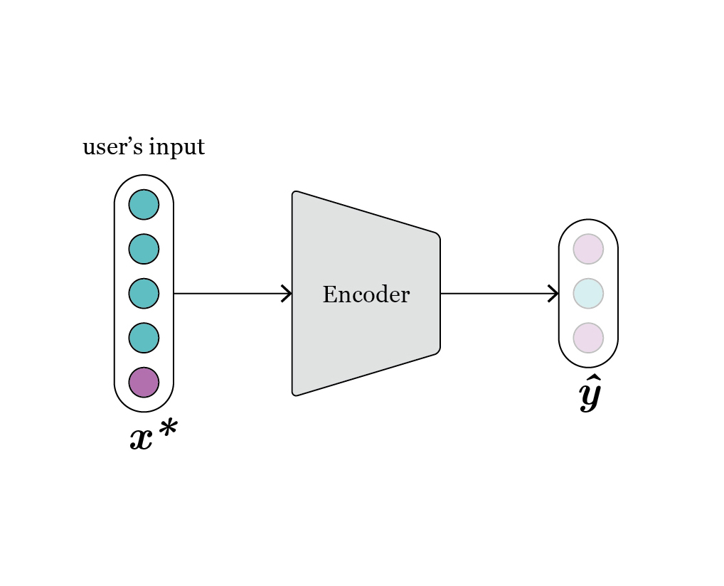
Fig. 5: depiction of the forward evaluation process.

Inverse design and generation

Through the Generator class we can perform inverse design, i.e. generate designs that fulfill values (of all or selected OutputML \(y\) variables) requested by the user.

Internally, the Generator carries out several steps, explained later in detail. These are handled internally, and transparent to the user. To use the Generator, the user just needs to first declare it, providing a model and a DataModule as follows:

from aixd.mlmodel.generation.generator import Generator

gen = Generator(model, datamodule, fast_generation=True, over_sample = 10)

When the Generator is instantiated, it prompts a message indicating which attributes can be requested, and the names to use. These requests can be formulated using different formulas:

# Given two attributes, y1 of dimensionality 1, and y2 of dimensionality 3, all the following requests are similar
request = {"y1": 5, "y2_1": 7}
request = {"y1": 5, "y2": [None, 7, None]}

# And for some given ranges, instead of fixed values
request = {"y1": [4,6], "y2_1": [6,8]}
request = {"y1": [4,6], "y2": [None, [6,8], None]}

As we can observe, we can request both specific values or acceptable ranges for the requested attributes. The former obviously defines more restrictive requests. Besides, the more attributes we request, the more prone the generated designs will be to deviate from the desired values.

Once defined a request, we just need to call the generator as follows:

xy, all_results = gen.generation(request, n_samples=10, format_out="df", print_results=True)

The method prompts a message with an overview of the results, in terms of the errors incurred for the number of samples requested, for a 10% of the best samples, and for the best sample.

# Error during generation

• Errors when requesting: sun_occlusion = [20.0, 30.0], surface_platf_1 = [35], surface_platf_3 = [50]

• Mean for 10 samples: 0.0, 0.66272086, 0.9577557

• Mean for 1.0 sample(s): 0.0, 0.4821968, 0.39183807

Best sample: 24.619483947753906, 34.51780319213867, 50.39183807373047

Besides, variable df_out combines the generated designs \(x\) with the requested values \(y\). If there is a direct mapping between InputML and DesignParameters, this can be fed to the CAD or FEM software for further evaluation.

Furthermore, all_results is a dictionary containing all the results derived from the internal operations of the Generator. Per se it is not useful to the user, but it can be harnessed by other methods. In particular, the plotter contains a method that allows to more visually represent the generated samples. For example, we can provide the output of 3 different requests as follows:

plotter = Plotter(dataset, model=cae, datamodule=datamodule, output='show')
plotter.generation_scatter([dict_results1, dict_results2, dict_results3], n_samples = 2)

Leading to the following plot:

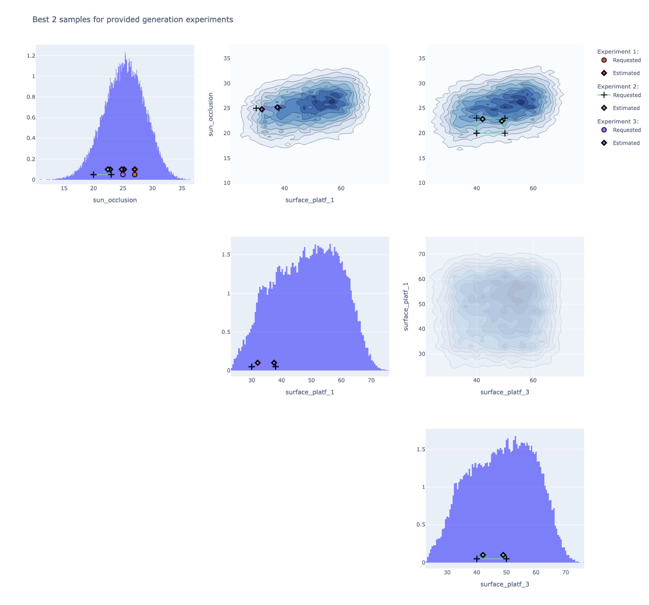
This plot results from the use case Semiramis, and the attributes requested are the sun oclussion, and the surfaces for platform 1 and 3. However, the request are different in each case:

request1 = {"sun_occlusion": 27}
request2 = {"sun_occlusion": [20,23], "surface_platf_3": [40, 50]}
request3 = {"sun_occlusion": 25, "surface_platf_1": [30, 38]}

We can observe then in the plot how each sample is just plotted in some particular contour plots and histogram, those that correspond to the attributes requested. This graph provides a visual representation of the performance of the generated geometries, and may allow understanding more in detail the behavior for more challenging requests, e.g. closer to the edges of the attributes’ distribution, where the model has observed less data during training.

As indicated before, all processes are abstracted into the Generator, to simplify its usage. In order to allow the user understanding fully the operations carried out, in the following we detail the full process. The reader can refer to Fig. 6 for a visual representation of the process:

• The Generator receives the request \(y^*\) from the user, which corresponds to some specific attribute(s).

• If the requested attributes are just a subset of all OutputML, the remaining attributes are sampled conditioned on the requested values. For this, a KernelDensityStrategy (mode details in sampler) is utilized, fit on the training split of \(y\).

• The decoder requires a full vector \([y,z]\). Hence, samples of \(z\) are also required.

  • For the CondAEmodel, i.e. the non-variational version of the AE architecture, these \(z\) vectors need to be sampled conditioned on each respective \(y\). This is a time demanding process that can be overridden by setting the flag fast_generation equal to True. Then, \(z\) is sampled from a zero mean and unit variance Gaussian, which may cause the generated designs to deviate more from the values requested.

  • For the CondVAEmodel, \(z\) is just sampled from a zero mean and unit variance Gaussian, as required by this specific archicture.

• Internally, more samples are generated than those requested. This is controlled by the parameter over_sample. Therefore, this leads to more designs being generated by the decoder, \(\hat{x}\).

• Among all designs generated, \(\hat{x}\), the best ones are selected using the design error calculated by the encoder, which acts as a surrogate model.

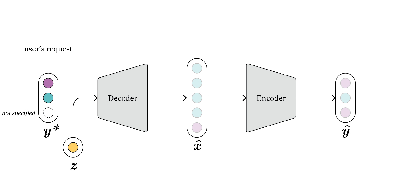
Fig. 6: intuitively, we can swap the position of the encoder and the decoder, as now first the decoder is used to generate new designs, given a request, and the encoder selects the best among all.

References

[Kingma2013]

Kingma, D. P., & Welling, M. (2013). Auto-encoding variational bayes. arXiv preprint arXiv:1312.6114.

[Sohn2015]

Sohn, K., Lee, H., & Yan, X. (2015). Learning structured output representation using deep conditional generative models. Advances in neural information processing systems, 28.

[Keskar2016]

Keskar, N. S., Mudigere, D., Nocedal, J., Smelyanskiy, M., & Tang, P. T. P. (2016). On large-batch training for deep learning: Generalization gap and sharp minima. arXiv preprint arXiv:1609.04836.